Final Prediction

November 1, 2020

This forecast uses polling numbers as of 3 PM EST on 11/1/2020.

Overview

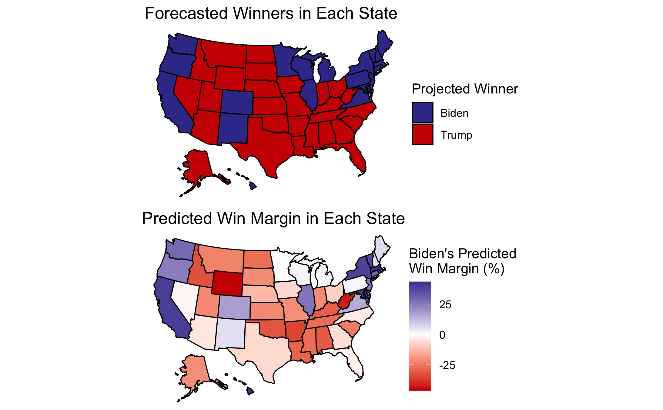
This forecast predicts that Joe Biden will win a popular vote victory of 52.7% with a narrow Electoral College majority of 273 votes compared to Donald Trump’s 265 votes. However, the model projects a high level of uncertainty in several battleground states. As a result, the Electoral College could easily swing to a Trump victory or further in Biden’s favor.

Model Description and Methodology

In this forecast, a binomial logistic model¹ predicts the state-by-state probabilities that an individual will vote for either party, using a combination of polling, economic, demographic, and incumbency data:²

To gauge public opinion, the model includes average state-level polls³ in the final 4 weeks before the election. Election-year Q1 GDP growth captures the state of the economy, and the incumbency term accounts for the incumbent advantage. Since past elections serve as excellent predictors for future elections, the forecast includes a term for the difference between Democratic and Republican state-level two-party vote share in the previous election. Lastly, demographic variables⁴–the change in the state’s Black population, age 20-30 population, and age 65+ population–capture the impact of shifting demographics on election outcomes. The Appendix includes a graph of the model’s coefficients, further discussion about each variable, and a more detailed description of how I arrived at my prediction from this model.

Out-of-Sample Validation

To test the validity of this model, I performed leave-one-out cross-validation for each state in every election from 1992-2016.

For example, I constructed a model excluding Texas in 1996 and then used that model to predict the winner of the Texas popular vote in 1996. I repeated this process for all 50 states across every presidential election from 1992-2016. Then, I compared each state’s predicted winners to the actual winners.

In elections from 1992-2016, this model correctly classified the statewide popular vote winner 92.2%⁵ of the time, with the following year-by-year breakdown:

Year	Correct Classification
1992	0.8260870
1996	0.9583333
2000	0.9130435
2004	0.9534884
2008	0.9782609
2012	0.9500000
2016	0.8800000

Not surprisingly, the model performed most poorly in swing states. Across all elections from 1992-2016, the model correctly classified the popular vote winner less than 75% of the time in these 6 states:

State	Correct Classification
FL	0.5714286
GA	0.7142857
NC	0.7142857
NH	0.7142857
PA	0.7142857
WI	0.7142857

In the leave-one-out validation for 2016, the model misclassified 6 states: FL, OH, NC, MI, PA, and WI. FiveThirtyEight’s 2016 forecast correctly predicted OH but misclassified the remaining five of those six states. Inaccurate polling numbers likely played a role in the misses for 2016. For the 2020 prediction, I aim to combat this by applying a weighting scheme that favors high-quality pollsters over less reliable sources.³

2020 Prediction

This model predicts a narrow Biden victory in the Electoral College, with a much larger margin in the popular vote:

Candidate	Electoral Votes	Two-Party Popular Vote
Joe Biden	273	0.5271979
Donald Trump	265	0.4728021

This table contains all state-level predictions of the two-party popular vote.

Uncertainty Around Prediction

Any model, including this one, has a near-zero probability of predicting the exact outcome of an election. However, forecasts provide insights into the range of possible election outcomes and the surrounding uncertainty.

As visible in the map of Joe Biden’s predicted win margin, this forecast anticipates close elections in many states, making a Biden landslide possible in the Electoral College if several of Trump’s close states flip to blue. On the contrary, Trump could win the Electoral College if some of the slightly blue states flip to red. How can we quantify the uncertainty with this forecast?

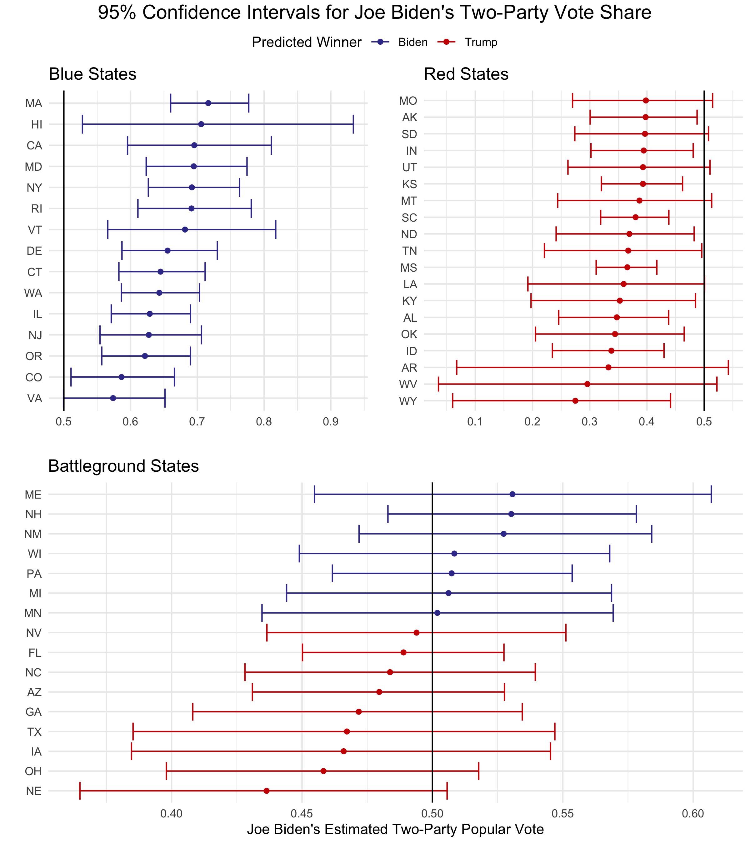
Confidence intervals serve as a helpful tool to measure statistical uncertainty. The below plot displays 95% confidence intervals for Joe Biden’s two-party vote share in each state. If a state’s interval does not contain 50%, then the forecast estimates with 95% confidence that the specified candidate will win that state’s two-party vote:

Moving away from estimated vote share, the remaining probabilities in this section do not represent vote share estimates; rather, these probabilities represent each candidate’s chance of victory. From 100,000 election simulations, this model gives Joe Biden a 62.8% chance of winning the Electoral College and Donald Trump a 35.1% chance of winning the Electoral College, with a 2.1% chance of an electoral tie:

Probability of Biden Electoral College Victory	Probability of Trump Electoral College Victory	Probability of Electoral College Tie6
0.62802	0.35074	0.02124

However, Donald Trump has a much smaller chance of winning the national popular vote:

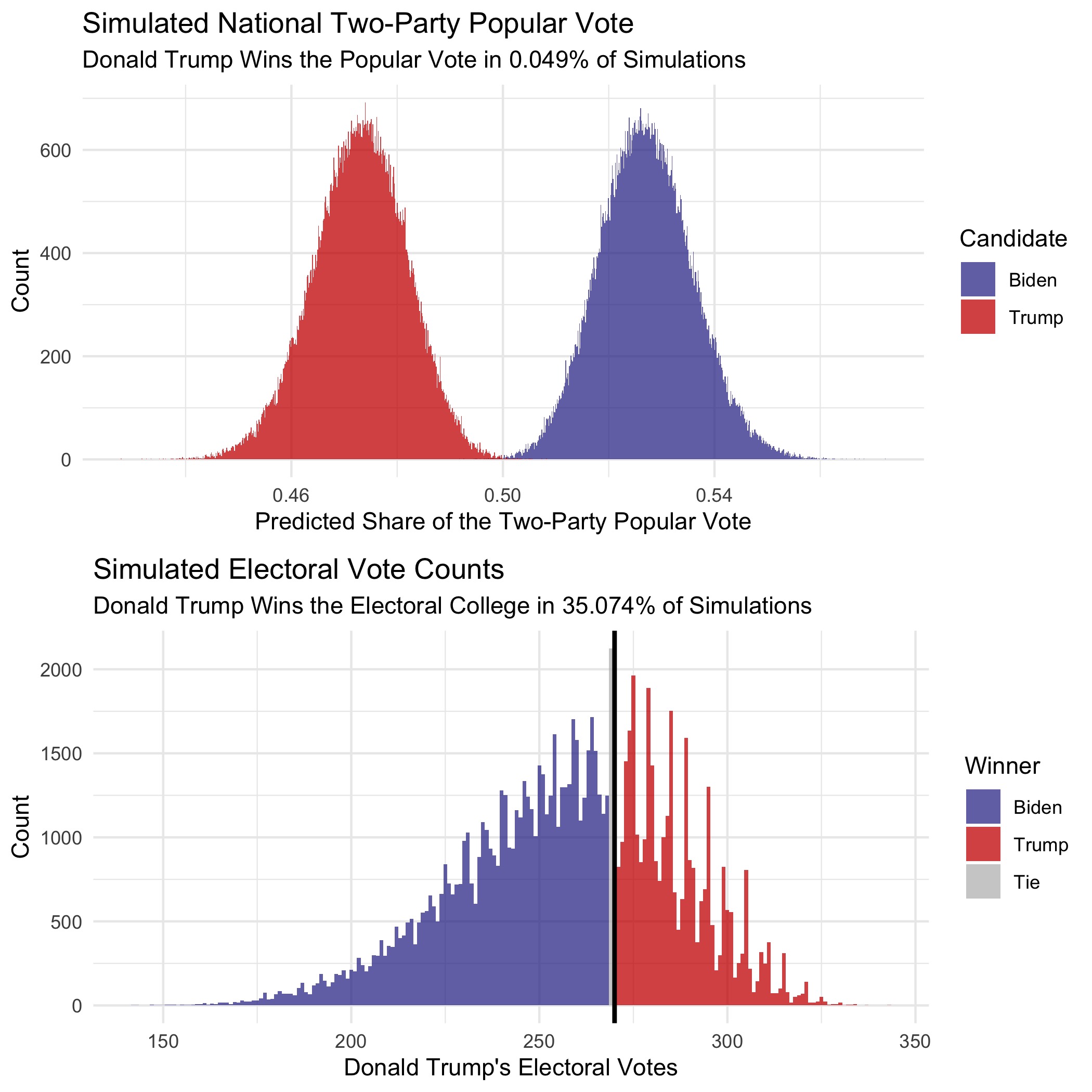
Luckily for Trump, the national popular vote does not matter if he can reach 270 Electoral College votes via statewide victories. While the forecast has a narrow Joe Biden victory as the point prediction, either candidate could reasonably win most of the battleground states. The below table lists the candidates’ probabilities of winning each battleground state, ordered by the projected level of uncertainty:

State	Probability of Biden Victory	Probability of Trump Victory
MN	0.5362000	0.4638000
NV	0.4394318	0.5605682
MI	0.5861000	0.4139000
FL	0.3125000	0.6875000
WI	0.6144000	0.3856000
NC	0.2859000	0.7141000
IA	0.2414000	0.7586000
TX	0.2090000	0.7910000
AZ	0.2047000	0.7953000
PA	0.6379000	0.3621000
GA	0.1921000	0.8079000
OH	0.0790000	0.9210000
NE	0.0439000	0.9561000
NM	0.7787000	0.2213000
ME	0.8016000	0.1984000
NH	0.9101000	0.0899000

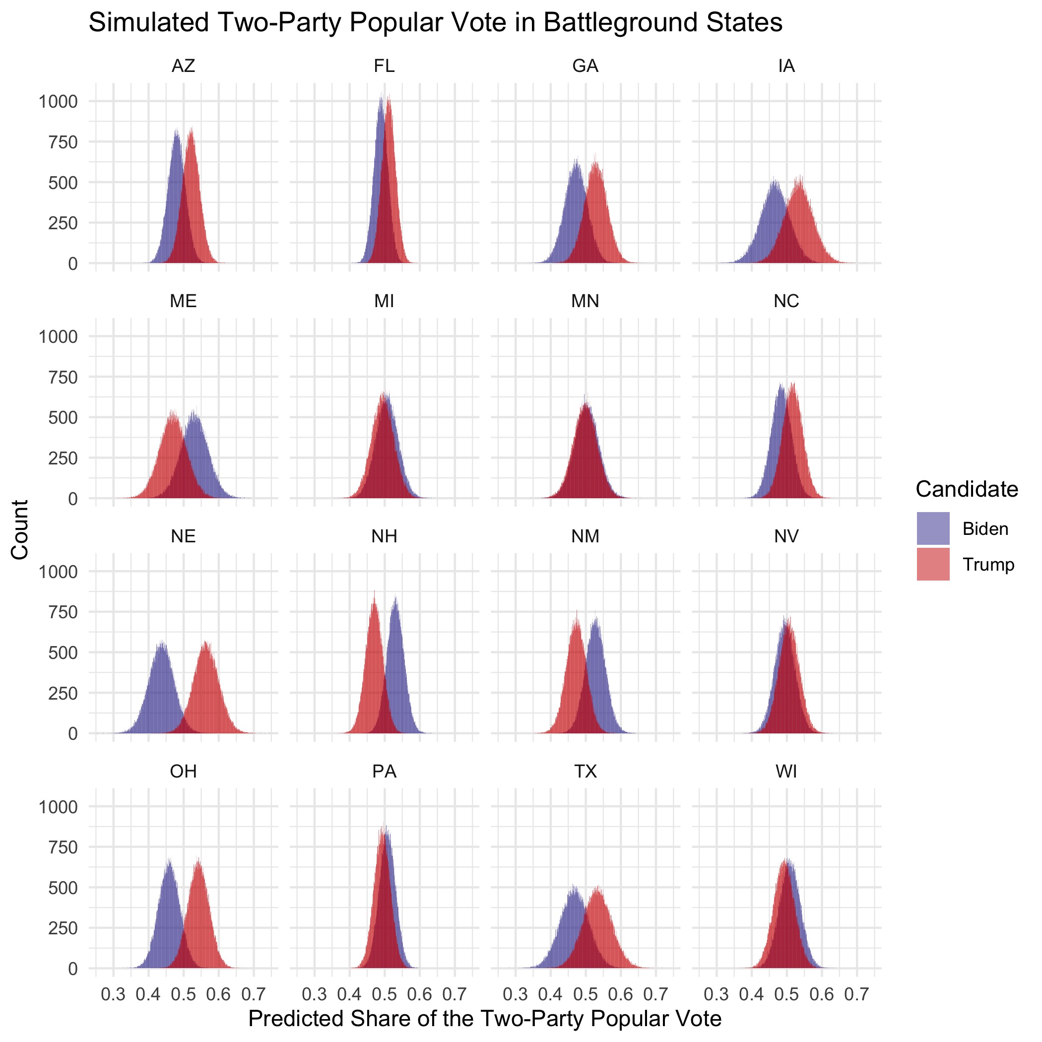
According to this model, the closest battleground races are fairly evenly split between the two candidates. However, these states could all easily swing in Donald Trump’s favor, giving him the Electoral College victory while still losing the popular vote. If one of Minnesota, Michigan, or Florida flip and the other states remain the same, Donald Trump will win the Electoral College. On the other hand, Nevada, Florida, North Carolina, and Iowa could easily all vote for Biden, giving him a much larger Electoral College victory than estimated by the forecast’s point prediction. For a more detailed look at each candidate’s state-level win probabilities, this table lists all states and corresponding levels of uncertainty.

Model Limitations

While this forecast performed quite well in the leave-one-out cross-validation and makes reasonable state-by-state predictions, it also has several limitations:

• This model does not account for Washington D.C. However, D.C. has a history of voting heavily Democratic, making it extremely likely to vote Democrat in this election. For this reason, Washington D.C.’s 3 electoral votes were added to Joe Biden’s Electoral College tally after allocating the votes from the 50 states.

• Due to the structure of the available data, this model treats Maine and Nebraska as winner-take-all states. However, these two states follow the congressional district method and can split their votes between candidates.

• The combined data⁷ for this model only dates back to 1992, which only allows for the model to fit itself with data from 7 previous elections. However, each state counts as an individual observation, increasing the total number of observations to 350. 105, 112, and 133 observations fit the blue, battleground, and red models, respectively.

• This model independently varies voter turnout and probabilities for each simulation.⁸ A more sophisticated model would introduce some correlation between subgroups such as demographics, COVID deaths, or partisan alignment. For example, low turnout among suburban women in Wisconsin would likely accompany low turnout among suburban women in Minnesota. While this forecast does simulate instances with lower-than-predicted probabilities of voting for either party within each state, the probability of voting for Biden in Wisconsin in a single simulation has no bearing on the probability of voting for Biden in Minnesota.

• To set a rule for how I classified states, I divided states into blue, red, and battleground states using the 2020 classifications by the New York Times. Unfortunately, this method does not account for the ideological evolution of states over time. For example, Texas reliably voted Republican in all other elections from 1992-2016, but the New York Times classifies as a “battleground state” for 2020. Ideally, I would have used historical Texas data to construct the “red state” model. If I did that, however, I would either have to (a) make judgment calls for each of the remaining 49 states in each of the 7 elections, or (b) set some other arbitrary rule for the year-by-year classification of states. In the end, I elected to follow the imperfect but uniform method of classifying states by their 2020 status.

Conclusion

This model predicts a narrow Democratic victory with a 273 to 265 Electoral College majority and approximately 52.7% of the two-party popular vote. However, the close state-level vote margins, especially in battleground states, increase the level of uncertainty.

Due to the close margins in several battleground states, the Electoral College could easily swing in the direction of a Trump victory or a Biden landslide. For example, if Joe Biden wins Michigan, Nevada, Texas, or any other state with a narrow victory projected for Trump, Biden could win far more than his projected 273 votes. However, if Trump wins New Hampshire, Nebraska, Pennsylvania, Wisconsin, or any other states projecting an extremely narrow Biden victory, he could easily tip the electoral scale in his favor. This forecast gives Joe Biden a 62.8% chance of a Joe Biden Electoral College victory, a 35.1% chance of a Donald Trump Electoral College victory, and a 2.1% chance of an electoral tie.

2020 has been quite the year, and the uncertainty surrounding the 2020 election will likely add to the chaos in the coming days.

---

Appendix

This section further explains the details of this model and expands upon ideas that did not fit well into the main content of this post.

Methodology and Steps-by-Step Breakdown

To create individualized models while avoiding overfitting, I grouped states into three separate categories: blue states, red states, and battleground states, as classified by the New York Times. Within each group of states, I constructed two models–one that predicts the probability of voting Democrat and one that predicts the probability of voting Republican–yielding a total of 6 models.

To convert the probabilities to actual vote counts within each state, I multiplied the probabilities generated by the model to each state’s voting-eligible population. I simulated 100,000 total elections for each state, with slight variations in voter turnout and voting probabilities each time.⁸

To produce a single value for the popular vote and Electoral College prediction, I had to aggregate the 5,000,000 simulations in some way. For the nationwide two-party popular vote, I took the average number of voters for each party within each state, then estimated the nationwide vote count by summing each party’s state-level averages. Using these two sums, I calculated the estimated two-party vote share for each party.

I assigned each state’s electoral votes to the candidate who won the popular vote in the majority of the 100,000 election simulations. Then, I summed the electors for each state and added 3 to Joe Biden’s vote tally to account for Washington D.C.

Discussion of Variables

State-Level Polls

A single nationwide race does not determine the winner of the presidential election, but rather, 50 state-level races combine to decide the winner. For that reason, this model makes use of state-level polling³ rather than nationwide polling. Donald Trump appears to fare better in state-level polls compared to nationwide polls, which makes this model predict a closer race than if it included national polls.

To account for the increased turnout in early voting, I included polling numbers from the last four weeks leading up to the election. This method yielded the best out-of-sample fit when compared to polling intervals ranging from the last five weeks to only the last week:

1. As election day nears, two contradictory phenomena occur: polls (a) converge to the election outcome, and (b) increase in bias due to herding toward the anticipated outcome. I included the last four weeks of poll numbers in an aim to strike a balance between the contradictory effects of accurate converging and biased herding.
2. Some states do not attract much attention from pollsters, so using polls from multiple weeks increases the number of observations and reduces the likelihood of skewed polling averages due to limited sample sizes.

Incumbency

Incumbent candidates benefit from structural advantages, including but not limited to increased media coverage, widespread name recognition, an early start to campaigning, and more. This model incorporates incumbency status to help capture the effect of incumbency status on vote share.

Q1 GDP

Data suggests that voters focus on the election-year economy at the polls as opposed to economic performance over the entire term of the incumbent.⁹ Assuming that a similar trend will hold for 2020, Donald Trump will likely face some punishment at the polls for the economy’s historic lows at the beginning of the COVID-19 pandemic. However, focusing solely on the Q2 economic numbers completely disregards the economic prosperity before the pandemic. On the contrary, using the extremely high Q3 numbers extrapolates in the other direction and minimizes the damage done by COVID-19. To balance between the highs and the lows, this model incorporates 2020 Q1 GDP growth. This metric is slightly negative due to the onset of the pandemic in the US in the final weeks of the quarter, but it is nowhere near as low as the Q2 metric. This metric more accurately reflects how I anticipate voters to assess the economy at the polls: not great, but not hopeless beyond return.

Previous Democratic Vote Margin

As mentioned in the main content of the post, past elections serve as one of the best predictors for current elections, especially at the state level. Incorporating each state’s previous Democratic vote margin considers recent voting behavior.

State-Level Demographics: Change in Black Population, Change in Age 20-30 Population, and Change in 65 and Over Population

Demographics serve as strong predictors for voting behaviors, so incorporating the change in each state’s Black population accounts for changing demographics in the voting population. Black voters in particular lean Democratic, so this variable captures potential shifts in the partisan leaning within each state. Also, age serves as a fair predictor of voting behavior: younger voters tend to vote Democratic and older voters exhibit a greater tendency to vote Republican. While conducting leave-one-out validation for models, this combination of demographic factors yielded the highest rate of classification success.

Coefficients

This table displays the coefficients for each model, the below figure plots the coefficients for each model. With near-zero p-values and incredibly narrow 95% confidence intervals, all coefficients are extremely significant:

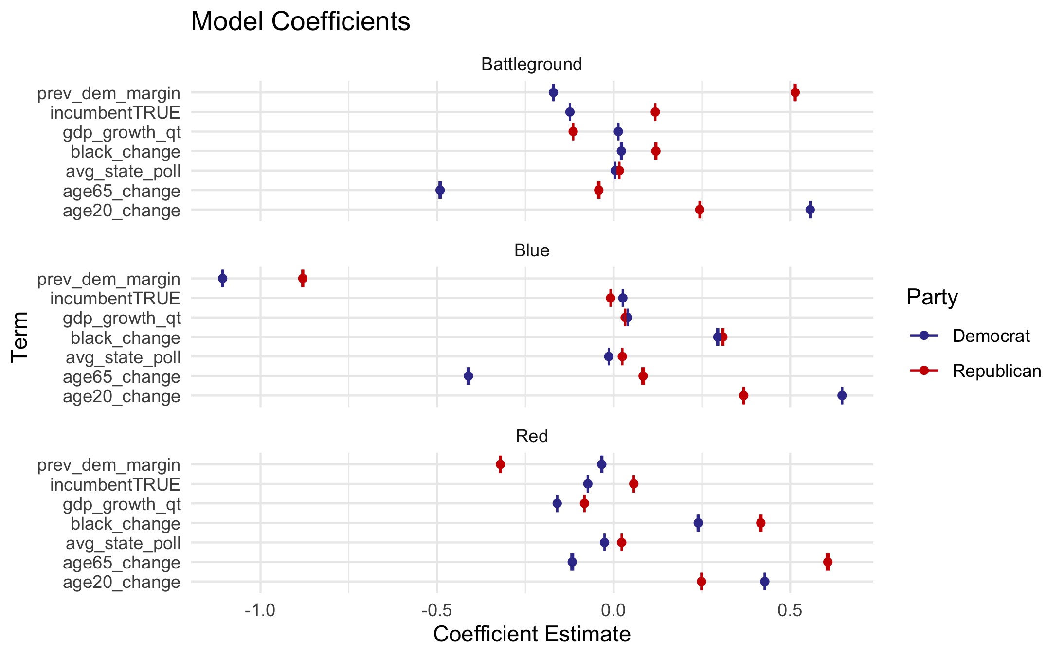
The above plot illustrates the differential effects of variables on the breakdowns of parties within state subgroups. For example, Q1 GDP growth and the change in the Black population has virtually the same coefficient for both parties in traditionally blue states. However, the change in the age 20 population within blue states has a greater positive coefficient for the Democratic candidate than the Republican candidate, and the change in the age 65+ population in blue states has a positive coefficient for republicans in blue states and a negative coefficient for democrats in blue states.

Other Notes

Downsides of Probabilistic Models

Well-known forecasting models give Joe Biden an extremely high probability of victory, with The Economist giving Biden a 95% chance of winning the Electoral College and FiveThirtyEight giving Biden an 89% chance of winning an electoral victory. Roughly 1 in 10 people confuse probabilistic forecasts with vote share estimates, so, while these forecasters do not have malicious intentions, their work often confuses voters. Probabilistic forecasts likely influenced turnout and played a role in the 2016 outcome in Donald Trump’s favor.¹⁰

The section on uncertainty of this post does mention win probabilities, but I prefaced the presentation of the numbers with a note that they are not estimated vote share. Humans naturally struggle with interpreting probabilities, so that forewarning may not have been enough. However, I felt that it was important to include the probabilities since they communicate that this model gives Donald Trump a decent chance to win the Electoral College.

Problems with the Electoral College

Nearly 3 million more Americans voted for Hillary Clinton in 2016 than voted for Donald Trump, yet he still won the election due to the United State’s Electoral College system. The win probabilities for both candidates in this forecast highlight the possibility for an electoral imbalance once again: Donald Trump has less than a 1% chance of winning the popular vote but nearly a 40% chance of winning the Electoral College. Many people argue that the Electoral College is an outdated system with no modern merits of existence. Unfortunately, the party reaping the advantages of the Electoral College system has resisted moves to strip them of their advantage throughout history, and that pattern will likely continue for the foreseeable future.

“Coming Home” and Polls in the Final Days

As Election Day approaches, voters appear to “come home” to their partisan loyalties in many states as close races become more spread out. Two weeks before the election, this model predicted that Trump would only win Texas by less than 0.01% of the popular vote, for example. However, it now gives Donald Trump an 80% chance of winning the state and forecasts a fairly decisive Trump victory in Texas.

In the FiveThirtyEight Podcast (released on 10/30/2020), Nate Silver described a tightening of polls in battleground states as the election approaches. Since most polls show a Biden lead, this should generally mean positive momentum for Trump. Does this indicate that some Trump supporters, previously apprehensive about supporting the president, are returning to their allegiances after all? Unfortunately, analyzing polls may only work to a certain extent. Can we trust polls to provide reliable information about voters’ positions, especially after they missed the mark by so much in the 2016 election? Luckily, only a few days of speculation remain before Election Day.

---

1. The g(x) in the model equation is a logit link function that models the probability of successes as a function of covariates. ↩

2. All data for this model is publicly available online. While many online sources host the data used in this model, the data for the 2020 state-level polls came from FiveThirtyEight, and the national GDP growth numbers came from the US Bureau of Economic Analysis. ↩

3. State-level polling in 2016 did quite a poor job of forecasting the election outcomes. Since this forecast uses state polls as the variable for public opinion, I aimed to exclude heavily biased or inaccurate polls where possible. To do this, I utilized FiveThirtyEight’s pollster ratings, which assigns grades ranging from A+ to D- to each poll. SurveyMonkey is one of only two pollsters with a rating of D-, but the platform issues the most polls out of anyone–nearly ten times as much as the second most prolific pollster. This pairing of low quality and high quantity makes SurveyMonkey polls incredibly problematic. To account for this, I applied an aggressive weighting scheme in an attempt to “crowd out” the low-rated polls. In calculating the polling averages, I counted A-rated polls 40 times, B-rated polls 20 times, C-rated polls 10 times, and D-rated polls 1 time each. Some states have a shortage of high-rated polls, which does not allow me to exclude low-quality polls altogether. This weighting scheme allows me to use the same technique for every state. ↩ ↩² ↩³

4. I only had state-level demographic data for the years 1990-2018, so I used the 2018 state-level demographic numbers to produce each party’s 2020 vote count projections. The change of the state’s demographics, as used in the model, accounts for the difference from the previous year’s percent composition of that state’s population. For example, if Alabama’s population was 75% white in 1990 but 74.8% white in 1991, the change in the white population for 1991 would be 0.2%. ↩

5. Not all states had enough state-level polling data to conduct the out-of-sample validation for each year; this percentage excludes NA values. ↩

6. This counts the proportion of times that neither candidate received at least 270 electoral votes. In the case of a tie, the House of Representatives would decide the winner of the presidential election. ↩

7. I could only find state-level demographic data dating back to 1990. Since this model uses state-level demographic variables, it could only fit itself with data from presidential elections from 1992 to the present. ↩

8. To vary the voting-eligible population (VEP) and the probability of voting for each party, I drew the values from a normal distribution. For the VEP, I used a normal distribution centered at each state’s VEP in 2016 and used a standard deviation of 1.25 times the standard deviation of the VEP in all years from 1980-2016. I multiplied the standard deviation by 1.25 because there will likely be more variability in turnout numbers this year; turnout could decrease in some states as a result of COVID-19 or issues with mail-in ballots, but turnout could also increase, as seen in historic early voting turnout in Texas. To simulate fluctuations in the probability of voting for each party, I took the absolute value of a draw from a normal distribution centered at the predicted probability for 2020 with a standard deviation equivalent to that party’s standard deviation of the two-party popular vote in the last three elections (2008-2016) within the respective state. ↩ ↩²

9. [Healy and Lenz, 2014] Healy, A. and Lenz, G. S. (2014). Substituting the End for the Whole: Why Voters Respond Primarily to the Election-Year Economy. American journal of political science, 58(1):31–47. ↩

10. [Westwood et al., 2020] Westwood, S. J., Messing, S., and Lelkes, Y. (2020). Projecting confidence: How the probabilistic horse race confuses and demobilizes the public. The Journal of politics. ↩